The long-run adjustment undertaken by a perfect competitive industry in response to demand shocks can result in increasing, decreasing, and constant cost, which then trace out long-run industry supply curves that are positively-sloped, negative-sloped, or horizontal, respectively.The path taken by an industry depends on underlying changes in resource prices and production cost. If the expansion of an industry causes higher resource prices and production cost, then the result is an increasing-cost industry. If expansion causes lower resource prices and production cost, then the result is a decreasing-cost industry. If expansion has no affect on resource prices and production cost, then the result is a constant-cost industry.
Demand Shift
| The Zucchini Market |  |
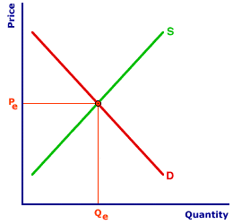
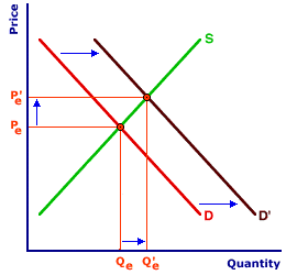
The perfectly competitive Shady Valley zucchini market can be used to illustrate all three alternatives. The original market equilibrium is presented in the exhibit to the right, with the supply curve S and the demand curve D. The market equilibrium price is Pe and the equilibrium quantity is Qe.The first step in identifying the long-run industry supply curve is an increase in demand. Click the [Demand Shift] button to illustrate the shift of the demand curve to D'. Note that with the increase in demand, the market price of zucchinis increases to Pe' and the equilibrium quantity rises to Qe'. The higher price and larger quantity is achieved as each existing firm in the industry responds to the demand shock. The higher price that buyers are willing to pay induces existing firms to increase their quantities supplied as they move along their individual marginal cost curves. The market, as such, moves along the original market supply curve from one equilibrium point to a higher equilibrium point.
However, the higher price leads to above-normal economic profit for existing firms. And with freedom of entry and exit, economic profit attracts kumquat, cucumber, and carrot producers into this zucchini industry. An increase in the number of firms in the zucchini industry then causes the market supply curve to shift. How far this curve shifts and where it intersects the new demand curve, D', determines if the zucchini market is an increasing-cost, decreasing-cost, or constant-cost industry.
Increasing-Cost Industry
| Increasing-Cost Industry |  |
Decreasing-Cost Industry |  |
Constant-Cost Industry |  |
First, consider how the zucchini market reacts if the entry of new firms causes an increase in production cost. The exhibit to the right illustrates this alternative.The entry of new firms into the zucchini industry shifts the supply curve to S', which can be seen with a click of the [Supply Shift] button. This new supply curve intersects the new demand curve, D', at the equilibrium price of Po and the equilibrium quantity of Qo.
The main point of interest is that the new equilibrium price is higher than the original. The reason that it is higher is that resource prices and thus the cost of production increase. One likely explanation is that the entry of new zucchini growers into the industry forces the price of one or more key zucchini-growing resources to rise. Perhaps the price of zucchini seeds rises. Maybe the price of zucchini fertilizer or zucchini shovels is higher. Whatever the actual resource price, the end result is the long-run average cost curve shifts upward. The minimum efficient scale for a given perfectly competitive firm is now at a higher cost.
To display the resulting long-run supply curve for this increasing cost industry click the [Long-Run Supply Curve] button.
Decreasing-Cost Industry
Second, consider the decreasing-cost alternative. The exhibit to the right illustrates this alternative.The entry of new firms into the zucchini industry shifts the supply curve to S', which can be seen with a click of the [Supply Shift] button. This shift is much greater than in the previous example. This new supply curve intersects the new demand curve, D', at the equilibrium price of Po and the equilibrium quantity of Qo.
The key point here is that the new equilibrium price is lower than the original. The reason for the lower price is that resource prices and thus the cost of production decrease. One possible explanation is that the entry of new zucchini growers into the industry causes the price of one or more key zucchini-growing resources to fall. Once again, it might be a lower price for zucchini seeds or perhaps the price of zucchini fertilizer or zucchini shovels is less. Whatever the actual resource price, the end result is the long-run average cost curve shifts downward. The minimum efficient scale for a given perfectly competitive firm is now at a lower cost.
To display the resulting long-run supply curve for this decreasing cost industry click the [Long-Run Supply Curve] button.
Constant-Cost Industry
The last of the three alternatives is a constant-cost industry. The last exhibit illustrates this option. Once again, the entry of new firms in the industry triggers an increase in supply to S', which can be illustrated by a click of the [Supply Shift] button. And once again, this new supply curve intersects the new demand curve, D', at a equilibrium quantity of Qo.However, in this case the new equilibrium price is the same as the old, Pe. And the equilibrium price is the same because the entry of new zucchini growers has no affect on production cost or resource prices. The long-run average cost curve does not shift and the minimum efficient scale for a given perfectly competitive firm does not change.
To display the resulting long-run supply curve for this constant cost industry click the [Long-Run Supply Curve] button.
LONG-RUN INDUSTRY SUPPLY CURVE, AmosWEB Encyclonomic WEB*pedia, http://www.AmosWEB.com, AmosWEB LLC, 2000-2024. [Accessed: May 1, 2024].


